Growing tree on a randomized output space
The bottleneck of random forest on multi-label and multi-output regression tasks with many outputs is the computation of the impurity measure at each tree node for each possible split.
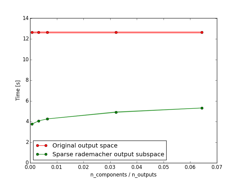
Growing a tree on lower dimensional random output subspace allow to decrease computing time while having the same or improved performance with a sufficient number of projections.

Python source code: plot_randomized_output_decision_tree.py
from __future__ import division
from time import time

import numpy as np
import matplotlib.pyplot as plt

from sklearn.base import clone
from sklearn.cross_validation import train_test_split
from sklearn.random_projection import SparseRandomProjection
from sklearn.metrics import label_ranking_average_precision_score as lrap_score

from random_output_trees.datasets import fetch_drug_interaction
from random_output_trees.ensemble import RandomForestClassifier

random_state = np.random.RandomState(0)

# Let's load a multilabel dataset
dataset = fetch_drug_interaction()
X = dataset.data
y = dataset.target  # y.shape = (1862, 1554)
X_train, X_test, y_train, y_test = train_test_split(X, y, test_size=0.5,
                                                    random_state=0)
n_outputs = y.shape[1]


def benchmark(base_estimator, random_state=None, n_iter=3):
    scores = []
    times = []
    for iter_ in range(n_iter):
        estimator = clone(base_estimator)
        estimator.set_params(random_state=random_state)

        time_start = time()
        estimator.fit(X_train, y_train)
        times.append(time() - time_start)

        y_proba_pred = estimator.predict_proba(X_test)
        y_scores = 1 - np.vstack([p[:, 0] for p in y_proba_pred]).T
        scores.append(lrap_score(y_test, y_scores))

    return scores, times


# NB: Increase the number of estimators to improve performance
n_estimators = 20

# Let's learn a random forest model
rf = RandomForestClassifier(n_estimators=n_estimators,
                            random_state=0)
rf_score, rf_times = benchmark(rf, random_state)

rf_score_mean = np.mean(rf_score)
rf_score_std = np.std(rf_score)

rf_times_mean = np.mean(rf_times)
rf_times_std = np.std(rf_times)

# Let's learn random forest on a Gaussian subspace
all_n_components = np.ceil(np.array([1, 5, 10, 50, 100]))
all_n_components = all_n_components.astype(int)
scores_mean = []
scores_std = []
times_mean = []
times_std = []

for i, n_components in enumerate(all_n_components):
    # First instatiate a transformer to modify the output space
    output_transformer = SparseRandomProjection(n_components=n_components,
                                                  random_state=0)

    # To fix the random output space for each estimator
    # Uncomment the following lines
    # from random_output_trees.transformer import FixedStateTransformer
    # output_transformer = FixedStateTransformer(output_transformer,
    #                                            random_seed=0)

    # Let's learn random forest on randomized subspace
    gaussian_rf = RandomForestClassifier(n_estimators=n_estimators,
                                         output_transformer=output_transformer,
                                         random_state=0)

    scores, times = benchmark(gaussian_rf, random_state)
    scores_mean.append(np.mean(scores))
    scores_std.append(np.std(scores))
    times_mean.append(np.mean(times))
    times_std.append(np.std(times))

scores_mean = np.array(scores_mean)
scores_std = np.array(scores_std)
times_mean = np.array(times_mean)
times_std = np.array(times_std)

# Let's plot the outcome of the experiments
fraction_outputs = all_n_components / n_outputs

plt.figure()
plt.plot(fraction_outputs, rf_score_mean * np.ones_like(fraction_outputs),
         "-o", color='r', label="Original output space")
plt.fill_between(fraction_outputs,
                 rf_score_mean - rf_score_std,
                 rf_score_mean + rf_score_std, alpha=0.25, color="r")
plt.plot(fraction_outputs, scores_mean, "-o", color='g',
         label="Sparse rademacher output subspace")
plt.fill_between(fraction_outputs,
                 scores_mean - scores_std,
                 scores_mean + scores_std, alpha=0.25, color="g")
plt.legend(loc="best")
plt.xlabel("n_components / n_outputs")
plt.ylabel("Label ranking average precision")
plt.show()


plt.figure()
plt.plot(fraction_outputs, rf_times_mean * np.ones_like(fraction_outputs),
         "-o", color='r', label="Original output space")
plt.fill_between(fraction_outputs,
                 rf_times_mean - rf_times_std,
                 rf_times_mean + rf_times_std, alpha=0.25, color="r")
plt.plot(fraction_outputs, times_mean, "-o", color='g',
         label="Sparse rademacher output subspace")
plt.fill_between(fraction_outputs,
                 times_mean - times_std,
                 times_mean + times_std, alpha=0.25, color="g")
plt.legend(loc="best")
plt.ylim((0., max(np.max(times_mean + times_std),
                  rf_times_mean + rf_times_std) * 1.1))
plt.xlabel("n_components / n_outputs")
plt.ylabel("Time [s]")
plt.show()
Total running time of the example: 175.47 seconds ( 2 minutes 55.47 seconds)